
|
AICVS hosted a session on Saturday, 7th of March, on Descending into Machine Learning. It was conducted by a very special speaker, Miss Nikita Kotak who works on technologies like Kubernetes, Docker, Google Cloud platform, Spring, Angular. She has studied Computer Engineering from P.I.C.T, Pune from the 2018 batch. She has worked on interesting projects in ML/AI domain during her academics and won few Hackathons and also published papers. Previously she has been a Google Applied CS with Android facilitator, Google Machine Learning crash course facilitator, Facebook Developer Circles Pune facilitator for Deep Learning and has also conducted a few Cloud training workshops. As of today along with her job,she likes contributing to open source projects and learning interesting new technologies. Artificial intelligence is a technology which enables a machine to simulate human behavior and machine learning is a subset of AI which allows a machine to automatically learn from past data without programming .She explained these basic concepts in an efficient way. The attendees saw the video of an AI assistant called Jarvis as well as the Amazon Go. Facebook CEO Mark Zuckerberg built an artificially intelligent, voice-controlled assistant for his home, Jarvis. Jarvis was designed by himself using Python, PHP and Objective C. He used open source artificial intelligence and machine learning projects created by Facebook and messenger platform too. Amazon Go is a chain of convenience stores in the United States operated by the online retailer Amazon. She showed the various implementations of ML and how AI and ML have largely affected the society as a whole. Christopher Olah's Blog and Andrew Ng’s Machine learning course are an excellent way to learn about these technologies as a beginner. A quiz was conducted regarding the previous concepts of models, labels and features. This quiz helped in clearing all the doubts related to Machine Learning. There was a lively discussion whether the questions in the quiz are true or false. It helped the beginners understand the reason behind answering the question and they also felt confident to discuss their views on the latest technology. Understanding the difference between a human mind and a machine was a key point in the session. The question is how much a machine can replicate a mind. Exactly simulating a human brain is simply not possible. With this given perspective, an algorithm has to be developed otherwise it will get unrealistic to train the model. Machine learning algorithms are very important for anyone who's interested in the data science field. Machine learning algorithms are quickly becoming a part of data to day business operations. Various machine learning algorithms like clustering, regression, classification and decision trees were discussed. Also, the gradient descent algorithm was talked upon. It is an optimization algorithm used in training a model. Gradient Descent finds the parameters that minimize the cost function. Minimizing errors and predicting the output closer to the actual answer are the benefits of this algorithm. Hands-on learning gives learners the opportunity to experience real world situations. There was a hands-on demo on how the gradient descent works. Active learning is a form of semi-supervised machine learning where the algorithm chooses which data to learn from and queries a teacher for guidance. Some examples of active learning were explored in the session. Pandas is an open source data analysis library for providing easy-to-use data structures and data analysis tools. Keras & TensorFlow are among the most popular frameworks when it comes to Deep Learning .The session was a hands-on workshop on Pandas and Tensorflow so basic introduction to Numpy and Panda was given in the talk. The topic of handling dataframes was explained and source codes were provided to the attendees. The session proved very beneficial to the beginners in the field of ML as it had no prerequisites.
2 Comments
Sri Harsha Gajavalli conducted a session on 22nd February 2020, on neural networks. It was aimed at the beginner audience with little or no knowledge of the topic. The talk started of with some fun binary question answer session involving the audience and was continued throughout the session, which held everyone's attention. 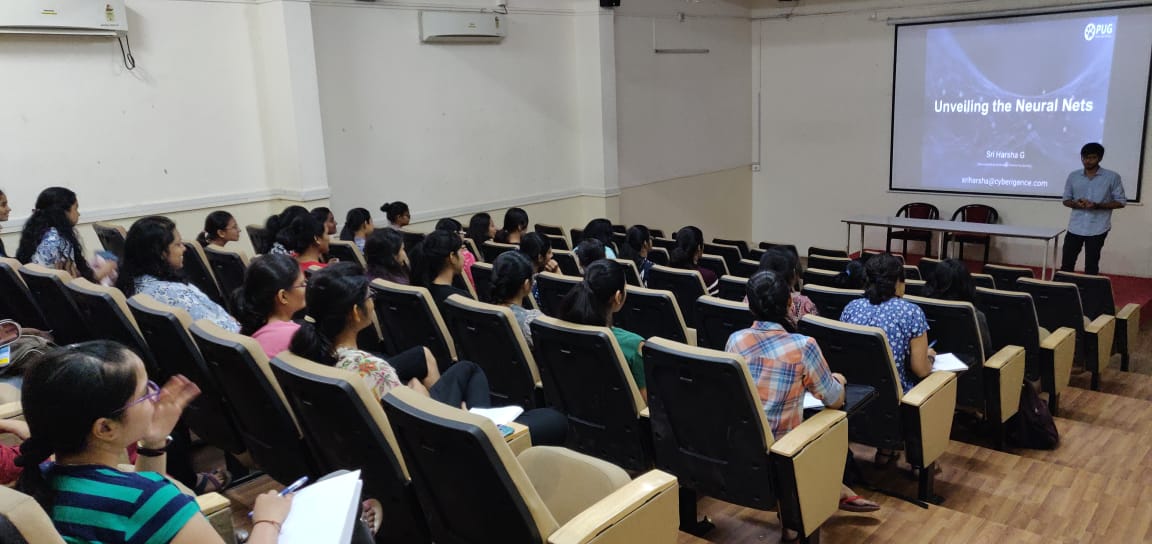 He began the topic stressing on the need of and the type of problems needing machine learning solutions. Justification for classifying a problem as a chine learning problem is a necessary first step. A simple way to find that out is to find out if you have a very large number of if conditions while trying to find solution to a problem. He further explained that the terms AI and ML have significant difference and cannot be synonyms. AI is used in decision making whereas ML is used for leaning from datasets. They are as different as learning and remembering are. An interesting example of biological neural nets is the pigeons as art critics experiment where pigeons are trained to differentiate between paintings of different artists. The best part being the high accuracy on testing them. ANN : They have 2 components - 1] nodes 2] weights Neural networks can only take numerical values as input data. So if you have categorical data, you have to express it as numeric data before proceeding to the neural network. The node has the structure: input -------> node (some hidden mathematical function) --------> output The hidden function can be an activation/squashing function. They are use to introduce non-linearity in the data which helps the network to provide accurate predictions as also to limit the output. The weight of the node helps to decide which feature is important. Feed Forward Net: Here the information flow is unidirectional. Data is passed to input layer, then to hidden layer and finally to the output layer. To select the right weight for a node, back propagation can be used. That is we start of with some small random weights and then calculate the error i.e. the difference between the predictions and the actual values and then adjust the weights to minimize the calculated error. This process of error minimization is known as gradient descent. The advantage of this approach is that it works relatively fast. But it needs a training set and at times can be extremely slow. Example for this can be voice recognition: recognize the voices of 2 persons A feed forward network is used and the following steps are repeated multiple times: 1] Present the data 2] Calculate error 3] Backpropagate the error 4] Adjust the weights Some of the applications of feed forward nets are: Pattern recognition, stock market predictions, sonar mine/rock recognition etc . Recurrent Networks: Here the data flow is multi-directional as the nodes connect back to other nodes or themselves. They are mainly used for language tasks. The differ from simple ANNs in context as they have a sense of time and memory of previous states. Convolutional Neural Networks: Here the kernels are used as local feature detectors. The main concept used here is that the neural network learns which kernels are most useful and then use these kernels across the entire data and then reduce the number of parameters and variance. Example of use of CNNs on image data: In case of an image, using kernels directly on the image excludes the edge pixels. Padding is used to avoid this effect. Stride is the step size of the kernel to move across the image. If the horixontal and vertical step-size is different, the output has reduced dimensions. In images there are multiple channels, i.e multiple numbers are associated with a single pixel location. The number of channels is known as depth. Kernel has the same depth as the image and each kernel outputs a single number at a pixel location. Pooling refers to shrinking dimensions of an image. There are different kinds of pooling operations like max-pool, average-pool etc. The session was a really interesting one and an important first understanding in entering the world of neural networks. Written by Manasi Khandekar.
 A session on Chatbot Development using RASA platform was arranged on 11th January 2020. It was conducted by Dr. Yogesh Kulkarni who is a former professor at COEP. He has 16+ years of experience in the software development field in various capacities and is currently the Principal Data Science Architect at Icertis , Pune. He taught about the development of a chatbot using RASA. The session started with a brief introduction about chatbots, IVR (Integrated voice response) and how chatbot solved the IVR problems. Advantages and disadvantages of chatbots were discussed too. For developing chatbot, natural language processing, machine learning and deep learning are the prerequisites. Gartner prediction – “85% of customer interactions will be managed without a human by 2020” Business Insider - “The global chatbot market is expected to reach $1.23 billion by 2025”  Chatbots are a form of human-computer dialog system which operates through natural language via text or speech. The backend of the chatbot is designed to handle messages from different channels and process them with Natural Language Processing (NLP) services. NLP is a subfield of linguistics, computer science, information engineering, and artificial intelligence concerned with the interactions between computers and human (natural) languages, in particular how to program computers to process and analyze large amounts of natural language data. Understanding Natural Language is Hallmark of Artificial Intelligence. NLU is a subpart of NLP. The type of chatbots are:-
 In the second half, the attendees were introduced to installation and usage of Rasa software. Rasa is an open source machine learning tool to develop text-and voice-based chatbots and assistants. Rasa NLU is an open-source natural language processing tool for intent classification, response retrieval and entity extraction in chatbots. It is written in Python. The reasons for choosing Rasa for development instead of several other platforms are:
- Written by Shreya Pawaskar.
In collaboration with Women Who Code Pune, we hosted Hacktoberfest , a day to celebrate open source software on 19th October 2019. A session on github was conducted by Sumit Kadu in the first half of the day. He is a principal engineer/ application architect with Mindbody technologies on Microsoft Technologies with an overall experience of 13 years in the IT industry. He took everyone through the history of git and also explained the git fundamentals. The second half was the hack time where the participants could contribute to python , ml or any other repositories, a list of which was carefully curated by the AICVS members. Parthvi Vala a guest speaker from Red Hat, concluded the session by reiterating the importance of contribution to open source projects.The enthusiastic participants received swags and goodies sent by Hacktoberfest and Digital Ocean.  The session on Git started with a brief introduction about version control system. A version control system tracks the history of changes made to a project as a team works on it. The conceptualization of git, its history and how it has evolved was discussed further, as also the advantages of using git. Git gives a unified view of a project and eliminates unnecessary work and avoids copies of the same project. Using github ,work is organized into repositories, where developers can outline requirements or direction and set expectations for team members. The developers can then work on the updates to the project by creating a branch and after its completion and approval by other team members, merge it into the main project. Key components in git are :
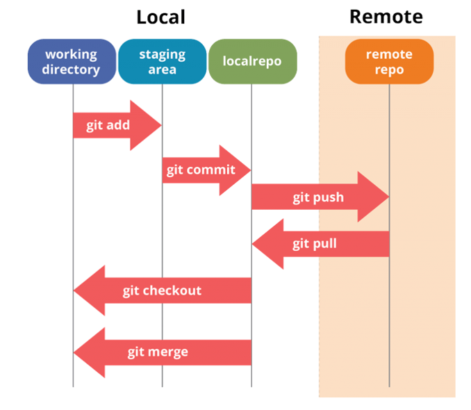 In order to use git, you can use certain specific commands to create , copy or make changes to codes. Basic git commands are :
The session concluded with a Q/A in which the thought provoking and different questions earned the questioner special goodies. The presentation on Git is attached below.
Written by Manasi Khandekar.
This is a hands-on tutorial on machine learning using OpenCV and Haar cascade classifiers. The tutorial will introduce you to Haar cascades and how to use these classifiers for face recognition and other object detection. By the end of this tutorial you will be able to train your own classifier for detecting faces and objects. 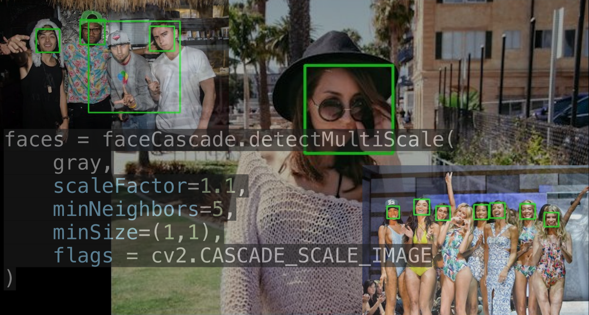 I’m writing this blog assuming that you have no prior knowledge of Machine Learning . Now, let’s talk about face detection. Face detection is finding one or many faces in a picture or a video. So, How do we find those faces? Well, we can use deep learning. Right? But actually the approach that everyone uses isn’t Deep Learning and it was developed in the early 2000s! Before deep learning was “a thing” to do everything :p, people used create algorithms with small neural networks, using machine learning and classifiers etc. and face detection was ongoing research at this time. In the year 2002, Paul Viola and Micheal Jones came up with a paper called ”Rapid Object Detection using a Boosted Cascade of Simple Features”. Here’s a link to the paper https://www.cs.cmu.edu/~efros/courses/LBMV07/Papers/viola-cvpr-01.pdf Here, I’ll attempt to explain their method in a simplified manner as to give you an insight to the concept of Haar cascades. Despite the fact that deep learning has taken over everything, this algorithm works absolutely fine till date! And if you have any kind of camera that does some sort of face detection, it’s probably using something very similar to this algorithm. 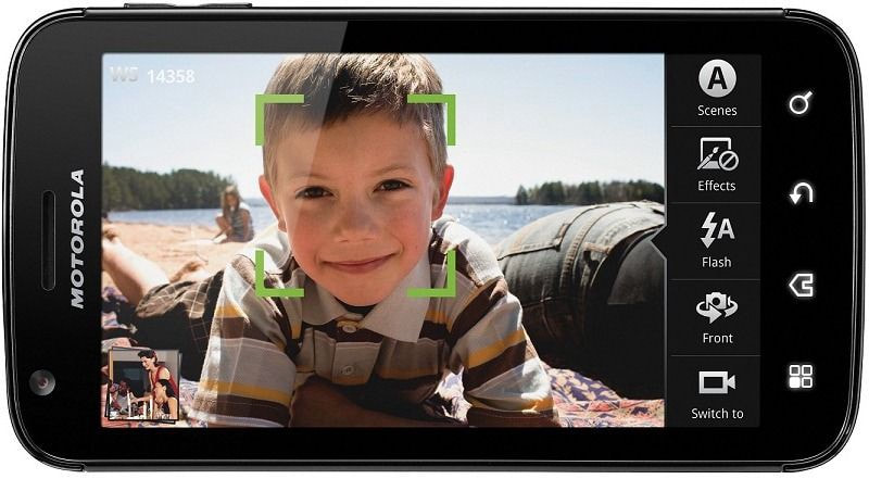 So what does this algorithm do? There are a few problems with face detection.
There’s a trade-off between accuracy and speed, false positives and false negatives and other constraints which makes it difficult to find faces quickly. Some other problems include the age, ethnicity, accessories such as if a person is wearing glasses etc. Viola-Jones came up with a classifier that uses very simple features that is one bit of an image, subtracted from another bit of an image. Unlike Deep learning which takes edges and other features and combines them together into objects, in a hierarchy and maybe it finds faces, what the Viola-Jones method does is it makes very quick decisions about what it is to be a face. \o_o/ For e.g. if you look at your own gray scale image, your eyes are arguably slightly darker than your forehead in terms of shadows and the pupils being darker. 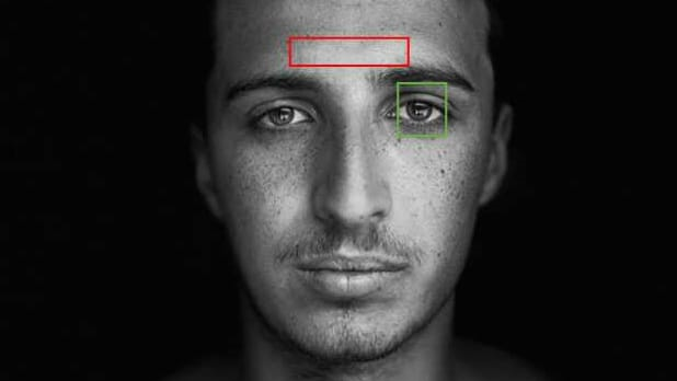 Hence the value of the image in the red rectangle subtracted from the value of the image in the green rectangle will produce a new different matrix. On its own this classification is very weak as it would also detect any other part of the image or in an different image where a certain section of the image is lighter than some other section. But if we could produce a lot of these all at once and make a decision that way. They proposed these simple rectangle features that subtracts one part of an image from another part. One of such features is a two rectangle feature. 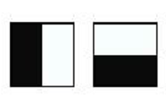 Voila-Jones algorithm is a machine learning approach. Since there can be many, say 500 faces in an image so we put in some features calculated from the image and we use machine learning to classify bits of the image or the whole image. Their contribution was a very quick way to calculate this features and use them to make a face classification. 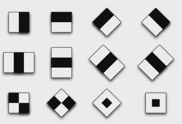 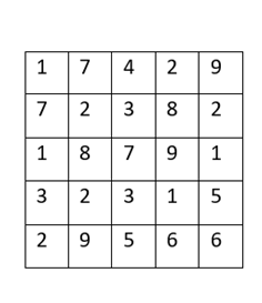 Their algorithm has a training process that selects certain features out of the many that makes sense in a particular section of the image i.e. to select the features that are useful. For e.g. a feature would be relevant over the eyes only and not anywhere else. Another problem is, on an image calculating large groups of pixels and summing them up is quite a slow process. So they came up with an idea called an integral image which makes this way faster. Suppose the given matrix is an image. (This is a very small image o_0,) Weight matrixSuppose we want to use the two-rectangle feature we previously discussed about : 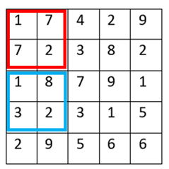 Suppose we want to use the two-rectangle feature we previously discussed about : Subtracting the blue block from the red block. That would be very simple: (Sum of the pixels in the red box) — (Sum of the pixels in the blue box) = (7+7+1+2) — (8+3+1+2) But, if you are doing this on a large section of an image and thousands of time this won’t work. Viola-Jones came up with Integral image where we pre-compute some of the arithmetic, store it in an intermediate form and then we can perform the rectangle feature function on it. 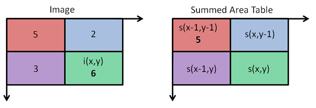 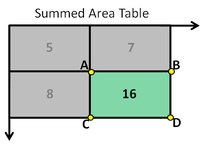 So we do one pass over the image, and every new pixel is the sum of all the pixels above and to the left and including it. Example of summed area table : For our image matrix 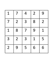 Integral Image would be 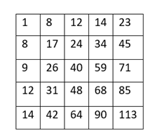 for eg: 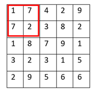 Sum of these 4 pixels 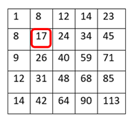 I’ll suggest you to do it for yourself , to understand it better. You’ll notice that in our sample image the sum of all the pixels is 113. 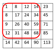 For e.g. the sum of the 4x4 block is 68 .So if we want to find the value of this region here 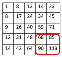 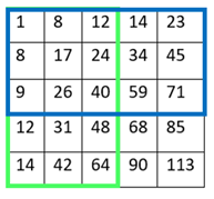 We would need to subtract the green box and the blue box. 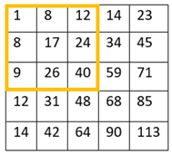 And add this bit, since it was subtracted twice.therefore, it would be 113–64–71+40 = 18 6+6+1+5 =18Since it’d be doing huge amount of calculations at once, the integral image is calculated once and then used as a base to do really quick adding and subtracting of regions. How does this turn into a working face detector? lets image we are detecting a face. In this particular algorithm we are looking at 24x24 pixel regions, but they can be scaled up or down a little bit. The algorithm calculates all 180,000 possible combinations of 2,3,4 rectangle features for that 24x24 pixel and work out which ones for the given data set (of faces and not faces), best separates the positives from the negatives. 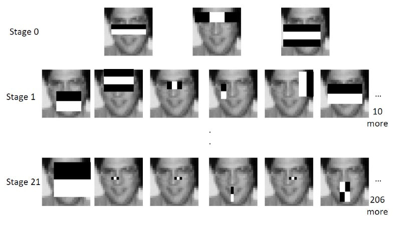 For e.g. In the image above, If all the features at stage 0 seem plausible, we let it through. If it fails to qualify in any of the three features in stage 0 we fail that region of the image. If stage 0 passes, we let it through the next stage. Which means the regions that passed the 0th stage, could be a face (but are definitely not NOT A FACE). Then all the regions that pass the 0th stage go through the stage 1 set of features and all the regions that pass through stage 1 go to stage 2 and so on. This is called a “Degenerate decision Tree.” Every time we calculate one of these features it takes little bit of time. The quicker we can say “no definitely not a face “, the better. And the only time we need to look through all these features (or all of the good ones) when we think that there actually could be a face in that region. So we can say less general, and more specific features go forward right up to about the number where we find a fail. And if we make it all the way to the end and nothing fails, that’s a FACE! Face Recognition using pre-trained Haar cascade classifiers. Here is a git-hub link to for various pre-trained Haar cascade classifiers https://github.com/opencv/opencv/tree/master/data/haarcascades These cascades are basically .xml files consisting of a lot of feature sets, and these feature sets correspond to a very specific type of object. Here, I’ll show you how to use some of these cascades and later we would discuss on how to make your very own cascade. We will be using the haarcascade_frontalface.xml and haarcascade_eye.xml files. Download these two files in the same project you would be writing your code in. import numpy as np import cv2 #Loading the two cascade files face_cascade=cv2.CascadeClassifier('haarcascade_frontalface.xml') eye_cascade=cv2.CascadeClassifier('haarcascade_eye.xml') cap =cv2.VideoCapture(0) while 1: ret, img = cap.read() gray=cv2.cvtColor(img,cv2.COLOR_BGR2GRAY) faces=face_cascade.detectMultiScale(gray, 1.3, 5) for (x,y,w,h) in faces: cv2.rectangle(img,(x,y),(x+w,y+h),(255,0,0),2) roi_gray = gray[y:y+h, x:x+w] roi_color = img[y:y+h, x:x+w] eyes = eye_cascade.detectMultiScale(roi_gray) for (ex,ey,ew,eh) in eyes: cv2.rectangle(roi_color,(ex,ey),(ex+ew,ey+eh),(0,255,0),2) cv2.imshow('img',img) k = cv2.waitKey(30) & 0xff if k == 27: break cap.release() cv2.destroyAllWindows() I’ll link a YouTube tutorial for the same. https://www.youtube.com/watch?v=88HdqNDQsEk Creating Your own custom Haar Cascade classifier A detailed step by step discussion on creating a Haar cascade has been discussed in this paper from University of Auckland (Link below), I do recommend you to try this approach on your own. https://www.cs.auckland.ac.nz/~m.rezaei/Tutorials/Creating_a_Cascade_of_Haar-Like_Classifiers_Step_by_Step.pdf I will also link a YouTube tutorial which uses Linux and AWS for training at a very low cost. https://www.youtube.com/watch?v=jG3bu0tjFbk But here, we will be discussing the more simple ,GUI approach for training which requires less time comparatively too. An Iranian developer named Amin Ahmadi has built this GUI (link) http://amin-ahmadi.com/cascade-trainer-gui/ That you’d be required to download. Now we need data sets for training there are many sources to find data sets, or you call simply download from google images. for face detection we will be using ck data set http://www.consortium.ri.cmu.edu/ckagree/  you need to form two folders n for negatives and p for positives. The p folder should contain all positives, in this case our positives will be faces. 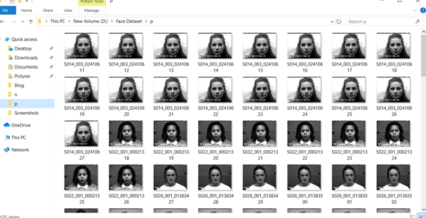 and the n folder should be negatives, in this case images with strictly no faces 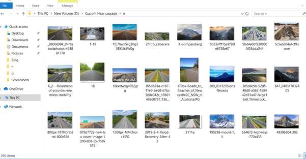 Once the data sets have been created you need to mention the path location of the data sets  Make sure that the data sets are named n and p. On the common tab, we can change the number of stages. With more number of stages, the time for training also increases but the model becomes more accurate too, in this case to train about 150 images 15 stages will be fine.  Keep the rest of the parameters at default.
On the cascade tab, you can change the width and the height, which is set at 24 (default). If you are using the ck data set, the images are bigger in size so we will set both sample width and sample height to 32. Keeping all the rest of the parameter at default, you can start the training process. Once the training is completed, you’ll see a classifier folder generated in your directory, which will contain a cascade.xml file. You can now import that file in your program and test your classifier. I strongly recommend you to try to create you own custom classifiers and test it. Also do visit the links and the tutorials for better understanding. |
|||||||
