|
The AICVS club hosted a competition based on Deep learning and computer vision on the Kaggle interface on 6th October, 2019. The participants were supposed to submit their entries from 00.00 a.m. to 11.59 p.m., after solving the dataset remotely on their laptops. The dataset provided was--"MNIST dataset for handwritten numbers ", a well-known, accessible dataset.
This competition was mainly meant for students with a certain level of understanding of Deep learning and Computer Vision. However, students of all years were strongly encouraged to participate in the contest, regardless of their proficiency in the subject. To facilitate the same, the participants were sent video links, educating them about visualization of the concept, implementation and neural networks. This ensured that they were well-equipped to start working on the dataset smoothly. The participants were allowed to use any approach to solve the dataset, whichsoever they found convenient. To elaborate about the dataset, the MNIST dataset for handwritten numbers is a dataset containing tens of thousands of small square 28×28 pixel grayscale images of handwritten single digits between 0 and 9 . The task for the contestants was to train the network to classify a given image of a handwritten number into one of the 10 classes representing integer values from 0 to 9,inclusively. MNIST ("Modified National Institute of Standards and Technology") is the de facto “Hello World” dataset of computer vision. Since its release in 1999, this classic dataset of handwritten images has served as the basis for benchmarking classification algorithms. As new machine learning techniques emerge, MNIST remains a reliable resource for researchers and learners alike. The participants were supposed to submit their classification along with a copy of their Jupyter notebook to curb plagiarism. Although many people registered for the competition and attempted to solve the dataset, some of them could not submit the output file. However, this was an incredible opportunity for learners to get their feet wet in Computer Vision and play around with various approaches to solve a single dataset. The winners of the competition-- 1st: Atmaja Jape | Score : 0.98906 2nd: Bhavana Mache | Score : 0.97640 3rd: Aathira Pillai | Score : 0.97146 The winners were calculated by Kaggle on the private (tested on 70% of the test dataset) and public (tested on 30%of the test dataset) leaderboards and was shared with the hosts. They would be awarded e-certificates. The competition saw the maximum participation from the CS and IT branches. The content of the competition was highly rated and the students found it exciting and innovative. We received feedback saying that the contest was held in a proper manner and the club members assisted every participant having queries promptly. Although some students faced issues in the submission of the problem and the Kaggle Notebook crashed many times due to ram. We have surely taken a note on this and we will make sure that we take steps to manage this issue. Kaggle is a great place to learn and to participate in data science challenges. It has helped students learn a lot of new things. The 'learning by implementing' way is a fun way to learn and was greatly appreciated by the participants. The competition gave an insight to various parts of deep learning. It was like a hands-on demo where participants could actually visualize data and find appropriate solutions. All the participants are looking forward to another such innovative competition. We received a 100 percent response for students interested in participating in another AICVS Competition and we will host that really soon. Till then keep learning and keep practicing! Written by Shreya Abhyankar and Shreya Pawaskar.
4 Comments
The AICVS club conducted an online machine learning competition on Kaggle platform on 14th September 2019 from 12 noon to 12 midnight. The participants were supposed to work on the dataset remotely on their devices. The competition used a very beginner-friendly dataset which is a popular choice for starting with machine learning--'The Titanic dataset'. Owing to a strong demand for hands-on projects by students, we decided to host this machine learning competition wherein even beginners with very little knowledge of ML models and a rudimentary knowledge of Python could tackle the problem statement using a step-by-step self-explanatory tutorial shared with the participants. The theme of the dataset takes its inspiration from the devastating shipwreck of Titanic. On April 15, 1912 during Titanic's maiden voyage, it sank after colliding with an iceberg, killing 1502 out of 2224 passengers and crew. Although there was some luck involved, some groups were more likely to survive than others, such as women, children, and the upper class. Based on the parameters -- Class of the passenger, gender, age, presence of the passenger's sibling, spouse or parents on board, fare, cabin and status of embarkment mentioned in the dataset the participants had to predict whether the concerned passenger survived the shipwreck or not. The participants had to submit their predictions along with a copy of their code on Jupyter notebooks to prevent plagiarism. The response to the competition was overwhelmingly positive with a total of 109 registered participants. The winners of the competition are: 1st: Mahima Malakwade 2nd: Aishwarya Keskar 3rd: Poorva Bhalerao who received an accuracy score of 0.87444, 0.87082 and 0.85897 respectively on the private(tested on 70% of the dataset) and public (tested on 30% of the dataset) leaderboards. Overall the contestants found the whole experience empowering and exciting. The Kaggle competition was a first ever kind of competition in the college which was related to the actual implementation of the datasets. It gave a hands-on experience to the beginners. A tutorial was given for helping even novices to participate and we ensured that everyone could access it easily. The topic chosen was found to very interesting by the contestants. We have received several requests to hold Kaggle or similar competitions at least every month. Exposure to ML and the quick replies to student’s queries on email by the committee were also highly appreciated. The students stated that it was the first time they used Kaggle, pandas etc. so they needed more time for the competition. Mostly the issues that the students faced were with the submission of the files and the interface was a bit difficult for the freshmen to understand . However we will make sure that we improve on these issues and provide them a better and more exciting event further. All the suggestions are appreciated and next time we will look upon how to make the competitions easier for the novices. The contestants have definitely liked this concept and we are sure that they will participate in the coming contests too. Even we guys enjoyed hosting the competition as much as the contestants enjoyed participating in it! The winner's python notebook submissions are attached below.
Written by Shreya Abhyankar, Aditi Jagdale and Shreya Pawaskar.
In this tutorial, you will learn how to complete the analysis of what sorts of people were likely to survive the Titanic shipwreck. In particular, you are going to apply the tools of machine learning to predict which passengers survived the tragedy. Description of Dataset The sinking of the RMS Titanic is one of the most infamous shipwrecks in history. On April 15, 1912, during her maiden voyage, the Titanic sank after colliding with an iceberg, killing 1502 out of 2224 passengers and crew. This sensational tragedy shocked the international community and led to better safety regulations for ships. One of the reasons that the shipwreck led to such loss of life was that there were not enough lifeboats for the passengers and crew. Although there was some element of luck involved in surviving the sinking, some groups of people were more likely to survive than others, such as women, children, and the upper-class. The steps we are going to follow to predict which passengers survived the tragedy: 1. Import data 2. Analyse the data 3. Data cleaning 4. Feature Selection 5. Model selection and training 1] Importing the Data Python Notebook Let us look at how we are going to load your dataset into a python file. You are probably using a Python IDE like IDLE to run your .py files. However, as seriousTM Machine Learning enthusiasts, we are going to use something that professionals use: Jupyter Notebooks. The Jupyter Notebook is an open-source web application that allows you to create and share documents that contain live code, equations, visualizations and narrative text. They’re used for data cleaning and transformation, numerical simulation, statistical modelling, data visualization, machine learning, and much more. If you want to load the data right now and start working with it, instead of having to install Python and then Jupyter Notebooks, no fear! You can also use Kaggle Notebooks! The screenshots below will help you open up a Kaggle Notebook in your browser. To install Jupyter Notebooks, follow the installation guide given on https://jupyter.org/ . 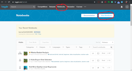 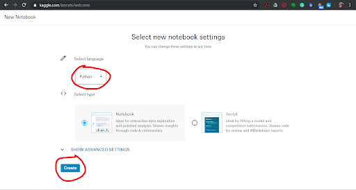 Adding the data We are now going to add dataset that we are going to use into the Python Notebook. 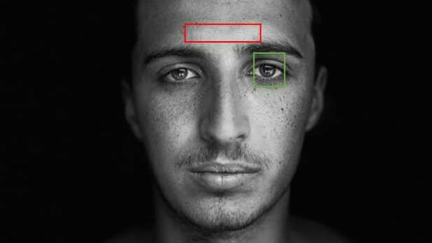 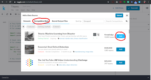 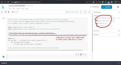 If you notice the dataset comes in two .csv files, training and test data. If you attended our session “How To: ML” by Ravina More, she explained the importance of splitting your dataset into training and test data. If you couldn’t attend the session, read this small article on it. Splitting your data is essential because you want to make sure your data is working correctly. But why not train your ML algorithm on all the data and test it on the same data? To have a real-world estimate of the accuracy of your model, we need to test it on data that it has never seen before. This is why we separate the data into training and test data. What do you think is the ratio of the split? Is it 50-50? Or is it 70-30? There exists another .csv file called gender_submission.csv which is a set of predictions that assume all and only female passengers survive, as an example of what a submission file should look like. Ignore that file for the time being. Loading data in Python Let us now load our dataset into our Python Notebook. We are going to use a Python library called Pandas. Pandas is the most popular Python library that is used for data analysis. We are going to be using a data structure in Pandas called DataFrames. Don’t worry about whether you know exactly what that is or not. Go ahead and look at the basics of Pandas from this site. Instead of spending all our time going through data frames and how to manipulate them, we’re going to jump right in and start working with it. First, import the pandas library with this statement. import pandas as pd Now let us look at how to load a .csv file in pandas. Google and search for the function to do this and save your loaded .csv files into two variables, train and test. train_df = #your code here test_df = #your code here Note: If you are getting an error in this step, consider that it might be because your filenames are wrong. If you run the lines underlined in red in the last screenshot, you will see an output that is a list of 3 file paths. Copy the relevant file paths into the function that you are using to load the data and it should work fine. 2] Analyse the Data Looking at the Data We shall now look closer at the dataset that we have just loaded to see what the data looks like. We have to figure out what we need to do with the data, what sort of algorithm to use, etc but we cannot do that until we can see what the data itself looks like. To do this we will analyse the whole dataset and for which we will temporarily combine the training and test data frames in a new variable called combine. We will not be performing our training on this dataset as we said before. combine = [train_df, test_df] We can also perform this analysis on the training data (train_df) only as well, but let us analyse the entire dataset. Analysis of the Data While analysing the dataset, let us try and answer the following questions: 1. Which features are available in the dataset?. 2. Which features are categorical? 3.Which features are numerical? 4. Which features are mixed data types? 5. Which features may contain errors or typos? 6. Which features contain blank, null or empty values? 7. What are the data types for various features? 8. What is the distribution of numerical feature values across the samples? 9. What is the distribution of categorical features? 1. Which features are available in the dataset? Let us print the entire data frame to see what it looks like. As you know already, to print a value in python, we have to just type the name of the variable on a new line. Hence, train_df will print the dataset and you will see the entire dataset at a single glance. 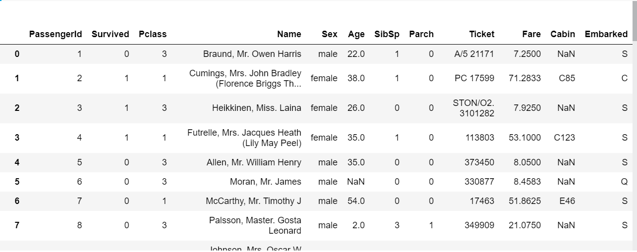 The features are the column names shown in bold (PassengerId, Survived, Pclass, Name, etc). These are called the features of the dataset and, as seen, is defined for every row in the dataset. Hence, each row is every passenger on the Titanic, or formally, every row is a sample in the dataset and each sample has features which are common across the dataset. NaN stands for not a number and can be interpreted as a value that is undefined or unrepresentable. Google and search for a command that shows the columns in a data frame. Your code should print out all the column names: 'PassengerId', 'Survived', 'Pclass', 'Name', 'Sex', 'Age', 'SibSp', 'Parch', 'Ticket', 'Fare', 'Cabin', 'Embarked'. There is an additional function of data frames that can be used to display a few samples in the dataset. Which function is this? 2. Which features are categorical? In statistics, a categorical variable is a variable that can take on one of a limited, and usually fixed number of possible values. For example, sex (not gender) can be of two types, male and female. A variable that can only take on values “A” or “B” or True or False, are also examples of categorical data. For this exercise, simply look through the dataset that you have printed and look at the values for each feature and note down the ones which you think are categorical. 3. Which features are numerical? Numerical data is data that take on numeric values. Note down the features that you think have numeric data. 4. Which features are mixed data types? Mixed data is a mix of numeric and alphanumeric data or simply alphanumeric data in the same feature. Note down the features that you think have mixed data type. 5. Which features may contain errors or typos? Think about this question as something to do with human error. Perhaps the person recording all the people who embarked on the Titanic was hard of hearing and sometimes wrote down the wrong thing. Which feature can be affected by this? 6. Which features contain blank, null or empty values? This information will be helpful to us when we are correcting the data. Look through the data for such missing values and note these features down. 7. What are the data types for various features? This can be useful when handling the data, for example, when adding in missing values, etc. We might say that the categorical, numeric and mixed data types are already something we know so why not use that data? However, here we are looking for specific Python data types. Google and search for ways to get columnar data types for data frames. To check your answer, the data type of PassengerId is int64. 8. What is the distribution of numerical feature values across the samples? Here we try to find various statistical measures in our features that can help us determine if the training data is actually representative of the problem statement that is trying to be solved. If it isn’t, our predictions will not perform well on the test data. We can apply several statistical measures like count, mean, standard deviation, min and max. We could spend our time writing code to go through each column of the data frame and returning the mean of that column, but that would be inefficient. The reason we are using pandas is because of its fantastic libraries. Try to find the function that would describe the distribution of numerical feature values for a data frame in pandas. It’s a single function that will return the values of count, mean, standard deviation, min and max, among others, for each column (also called feature) of the dataset. 9. What is the distribution of categorical features? If you noticed, the function used above is called on the entire dataset, but only returns count, etc for numeric data. To make it return categorical feature analysis as well include this in the parameter of the function. include=['O'] 3] Data Cleaning Missing Values We have seen that a number of features have missing values. The features that have null values are Age, Embarked and Cabin. Let us now see how we can complete these features. The number of missing values for each of these features can be found out by running the code given below. Find the number of missing values for each of the columns with missing values. print('Percent of missing 'column name' records is %.2f%%' %((train_df['column name'].isnull().sum()/train_df.shape[0])*100)) Age Feature One way to complete a feature is by assigning all the null values to randomly generated values. But that would introduce outliers (samples do not follow the pattern in the data and can cause us to make wrong predictions). So don’t do that. Another thing we can do is replace the missing values with the mean of the data sample ages that is already there. This would not change the mean or affect the dataset or pattern in the data greatly, so we go ahead with it. Let us now write the code for this: import math age_mean = #your code here num_rows = #your code here for i in range(num_rows): #basic for loop if math.isnan(#your code here): #your code here = age_mean train_df #to see the updated dataframe The functions that have been used for it can be found out by googling what you want to find and looking through documentation. Search for how you can find the number of rows in a dataframe, how to get the mean of a dataframe, or how to get the mean of a particular column, etc. Embarked Feature The embarked feature is a categorical feature that takes values either S, Q or C depending upon the port of embarkation. In the Age feature, we have replaced NaN values with the mean value. When we check the number of NaN values for the embarked feature, we see that it is quite less, 0.22% (Go ahead and check if you haven’t already.) Hence we can simply replace it with the most frequent value, ie, the port from which most people embark, as this would not change any pattern that the data is currently showing. If you remember correctly, this is another sort of measure called mode, ie, the most frequently occurring data sample. As in the above example we can use a loop to go through the “Embarked” column and if the value is NaN, we can replace it with the mode. However, there are better and more efficient ways to go about this. There is a function to fill only the NaN values in a dataset with a particular value (or set of values). Let us use that now instead. train_df["Embarked"]. #your code here(train_df["Embarked"].value_counts().idxmax(), inplace=True) If you go through the dataset now by printing it, you will see that values that were previously NaN are now filled up with the mode of ‘Embarked’. Cabin Feature Now let us look at the Cabin NaN values. When we look at the number of values that are missing in the Cabin we feature, we see that it is quite high, greater than 50%. It would be better to simply drop the column entirely than trying to come up with randomly generated values for these missing values. This is because if we fill it in with random values we may accidentally create or introduce some sort of pattern in the data that isn’t there or might increase variance. If this column is so incomplete, our ‘Survived’ column, ie, the one which says which passengers survived the Titanic disaster, probably does not depend on the ‘Cabin’ feature anyways and so it would be safe to drop it from our dataset entirely. Search how we drop columns in dataframes. train_df.#your code here(#your code here, axis=1, inplace=True) Now that we have cleaned our data, let us ensure that there are no missing values in the dataset, incase there is some feature with missing values that we have missed. Running the following code will show us if there are any more missing values in the dataset. train_df.isnull().sum() You should get a column on zero’s. Now print the train_df to look at your cleaned dataset! Categorical to Numeric Data Machine Learning models can categorize numeric data very well but often finds it hard to do the same with categorical data. This is because categorical data usually has words to represent a certain thing like ‘M’ for male and ‘F’ for female in the Sex column. Having categorical data in your model will cause an error message like “Your dataset has categorical data while your model requires numeric data” to pop up. This is why we need to convert our categorical data into numeric data. To do this we can simply, assign a number to each label, ie, the Sex column can be transformed into a rows of 1’s and 2’s with ‘F’ being assigned 1 and ‘M’ being assigned 2. However, it would be better to simply make a column, ie, you only need to know if a passenger is female or not. There is no need of a male or a combined Sex column. Thus, you transform the ‘Sex’ column into a binary column of 1’s and 0’s indicating if the Sex of the passenger is female or not. Similarly a column like PClass with 3 levels of classes can be split into 3 sets of columns, PClass_1, PClass_2 and PClass_3 which will have binary columns each, answering the question, “was this passenger in PClass 1?” This can be done with a function called get_dummies from the pandas library. Think about the feature columns that need to be transformed to numeric data (there are 3) and run the following code. You should also drop 'Sex_male' column since we only need one sex inticator. You already know how to drop columns. train_df = pd.get_dummies(train_df,columns=[#your code here]) #drop the 'Sex_female' column here train_df You will now see your dataset looks like this: 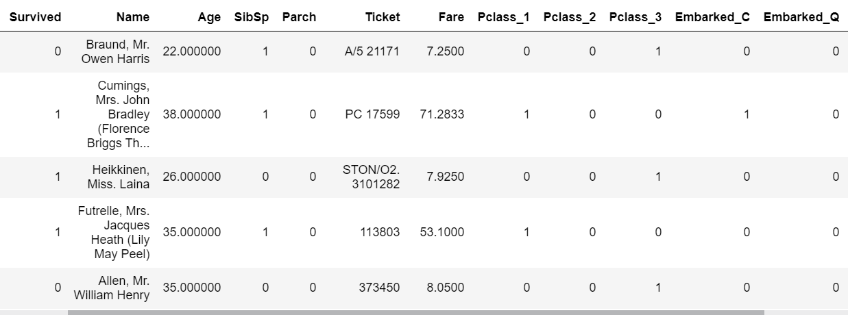 You see that there are Pclass has been replaced with 3 new columns of Pclass_1, PClass_2 and PClass3 and the same for Embarked. You have to apply these same transformations to the test dataset as well. This is because your model will be trained on a specific set of features and will expect the same features when testing the data. So apply all the data cleaning and converting categorical values into numerical values to the test dataset as well. 4] Feature Selection Dropping Features Let us now think about the features that we have in our dataset. There are 3 features that probably don’t affect our Survival rate. For example, “Name” would not affect if I survived the Titanic Disaster. Rose didn’t survive because of her name and neither did Jack die because of his name. We could probably drop the entire column and it would be fine. Figure out the two other features and drop them as well. You have already seen how to drop features. Adding Features Both SibSp and Parch relate to traveling with family. For simplicity's sake (and so that the same feature isn’t ‘counted’ twice, ie, multicollinearity), let us combine the effect of these two variables into one feature that says whether or not that individual was traveling alone. train_df['TravelAlone']=np.where((train_df["SibSp"]+train_df["Parch"])>0, 0, 1) Now drop the ‘SibSp’ and ‘Parch’ features from the dataset. You have to apply these same transformations to the test dataset as well. This is because your model will be trained on a specific set of features and will expect the same features when testing the data. So apply all the data cleaning and converting categorical values into numerical values to the test dataset as well. NOTE: Check for the missing values in the test_data carefully. There might be new features with missing values, in which case think about what has to be done. Now your data has been cleaned and we can move on to model selection, training and testing. 5] Model selection and training While analysing our data we have figured out that given a sample person’s data, we need to predict if he survives or does not survive the Titanic disaster. Notice that we aren’t being told to predict the probability percentage that he will survive the disaster. We simply have to say “YES” or “NO” to the question, “Did he survive the Titanic disaster”. There are various types of Machine Learning Algorithms but the algorithm that can be used here would belong to a class of algorithms called classification algorithms. Classification algorithms are used to answer Yes/No questions. Questions like: “Is this a human?”, “Is this a pen?”, and “Did this person survive the Titanic?” There are a number of Classification Algorithms we can use including:
You might be wondering how you will be able to implement these algorithms if you haven’t even heard their names before and especially if AICVS hasn’t even conducted any sessions on it. The beauty of Machine Learning and Python is that you don’t need to know the details of implementation to use an algorithm. Think of it like using a programming language. You learn a programming language like Java by learning how to write if-else statements, then how to write functions and classes and create objects, and so on. You might be an expert Java programmer but you still might not know how Java was created, or how your machine understands your Java code. But that’s because it does not matter to you, at that moment. You might know the specifics of programming language creation or compilers but that does not matter. In that same way, you need to know what the models and doing but it’s alright if you don’t know how they’re doing what they’re doing. Of course, as you go further into ML, you will and should, learn the specifics of each model and how they differ from each other and which model to choose over the others for a specific type of dataset. For now, however, let us treat them as black boxes. Python has very extensive libraries in which we can implement these algorithms with only a few lines of code. Let us look into the Logistic Regression model now and see how each performs after training, on our test data. Logistic Regression Logistic regression measures the relationship between the categorical dependent variable (feature) and one or more independent variables (features) by estimating probabilities using a logistic function, which is the cumulative logistic distribution. (Reference Wikipedia) Let us look at the Python code for Logistic Regression. We can also split our test and train datasets into X_test, X_train, y_test and y_train using train_test_split. from sklearn.model_selection import train_test_split X_train, X_test, y_train, y_test = train_test_split(train_df.drop('Survived',axis=1), train_df['Survived'], test_size=#your code here, random_state=101) We are importing the Logistic Regression model from the scikit-learn library. We are now going to create an instance of the logistic regression model. from sklearn.linear_model import LogisticRegression log_model = #your code here Remember that we had two data files, test and train. We’ve also previously explained why we need two files and cannot train the model on the whole dataset. Our model that we have just imported from the scikit-learn library is untrained and so we need to train the model on train.csv. Search how that would be done. log_model.fit(#your code here) Now that our model has been trained on our training dataset, let us test it on the test.csv data. This will help us understand how accurate our model is on new samples, ie, samples it hasn’t seen before. predict = log_model.#your code here(X_test) Now that we have a list of predictions on X_test and we have the “correct” predictions on that data, ie, “Y_test”, we can now find an accuracy score for our model. There are various metrics that we can use to see our accuracy including precision, recall and F1 score. We can calculate them at the same time using classification_report. from sklearn.metrics import classification_report print(classification_report(y_test,predict)) This will print out values of precision, recall and F1 score for 1 (survived) and 0 (did not survive). The accuracy row will give you your models accuracy (eg: 0.79 == 79%) Conclusion Now that you know how to go about fitting one model, why not try looking up how to fit other models? Better yet, take another dataset (there are hundreds available on Kaggle) and see if you can get the same accuracy level. Additionally look at other people’s solutions, videos and tutorials to see how to approach a dataset in different ways. Soon you will grow comfortable with tackling datasets and can take anything thrown at you. Happy Learning! Drop us an email at: [email protected] to tell us how you liked this tutorial on how to go about approaching the Titanic dataset or tell us if we can make any improvements that would make it easier for other beginners to tackle this dataset. Written by Michelle Davies Thalakottur. For our very first session, we asked an AICVS veteran, Ravina More to talk about the basics of machine learning and how to go about it taking a top-down approach. A system engineer at Tata Research Development and Design Centre (TRDDC), she spoke about getting started with ML, shared some "cheat sheets" and the importance of research for undergraduates.  She started off with the analogy of a human throwing balled up paper at the trash and how the accuracy of the throw improves after a few tries. This served as a good introduction to the definition of machine learning: “A computer program is said to learn from experience E with respect to some task T and some performance measure P, if its performance on T, as measured by P, improves with experience E.” --Tom Mitchell, 1997 Basically, the machine learns from experience of performing a task hence improving its overall performance (at performing said task).  In supervised learning, we split the data (usually 80:20) and train the first set, while leaving the second for testing. The trained model then works its charms on the test data and we gauge its performance accordingly.   Classification is used when we have categorical values (i.e. Non-continuous, non-numeric predictions). For example, we use classification in predicting presence of cancerous cells, or in predicting whether a loan application should be approved or not. Regression on the other hand, is for continuous (non-discrete) data. So, we use regression to predict house or airline prices. In unsupervised learning, no test data set is given to the algorithm and it must find its own understanding of mapping input to a desired output. Thus, in unsupervised learning, the algorithm must find all patterns in the data by itself. We looked at clustering in unsupervised data, which is when the machine finds similarities in the data and groups the data points in "clusters". Next, she spoke about overfitting and underfitting your model, both unwanted for good accuracy. In overfitting, the model is trained too much and hence acquires a bias for the given data points, making it inaccurate for newer data. Underfitting occurs when the model hasn't been trained enough and can't make adequately accurate predictions based on test data. Two students, Kinjal Parikh and Elice Priyadarshini then spoke about their experience with machine learning projects. You can find their blog here. Check out Ravina's presentation below:
 Written by Ruchi Pendse
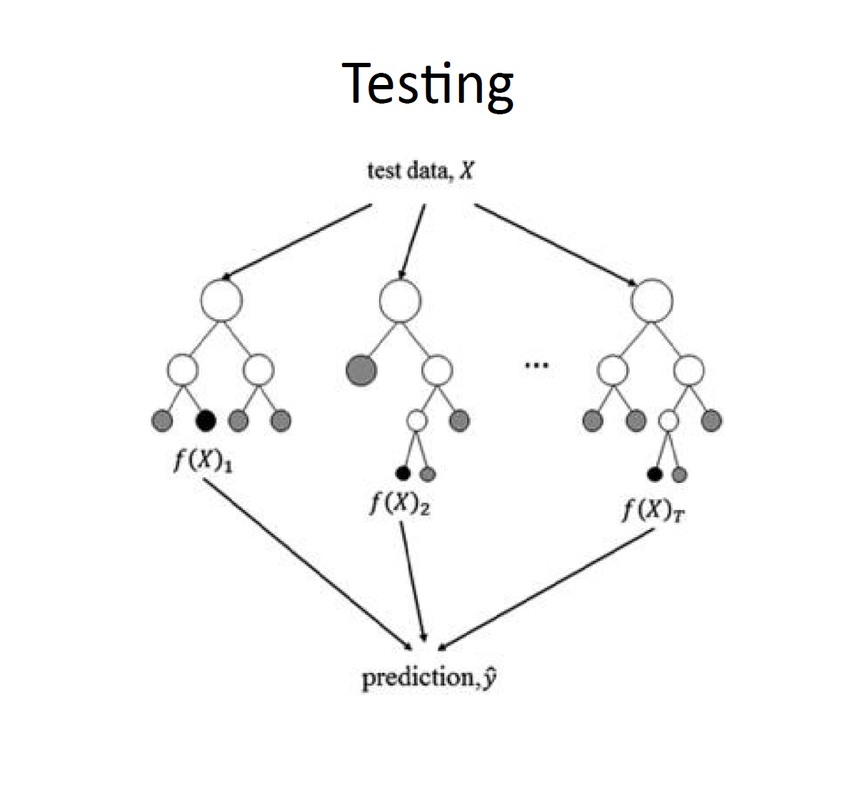
Ravina More conducted a session on 16th October, 2018 on Random Forest Classifiers.  Ravina More during the session Her talk started off with the basics of writing a code to train your model. The most important part is choosing an appropriate algorithm to train the model. Depending upon the need of our model we chose an algorithm which then shapes our entire model. In total there are four different methods available to choose - Classification, Regression, Clustering method and Dimensionality reduction. If your model is trying to predict the category in which a given sample will fall into, either Clustering or Classification algorithms are used. Classification is possible only when labeled data is available. If non labeled data is available then clustering method is adopted. However if your model is trying to predict a certain value and not a category, Regression or Dimensionality Reduction algorithms might be better suited for training your model . Regression is the method we use for prediction purpose. And if we want to create an apt data set out of available huge data then we use Dimensionality reduction algorithms. It is also used to identify and eliminate redundancies.  Choosing your learning algorithm In this session our main focus was Classification algorithms. Random forest classifier is a classification algorithm. Examples that fall under this category are Email Filtering, Face recognition etc. An example was then explained for us to get proper idea about how exactly the algorithm works. The example was – To Play Golf or Not. The features in the data set were – outlook, temperature, humidity, wind. The output that we need is “yes” or “no” to play. Among these variables it is important for the programmer to decide which variable is the deciding factor for our output. But to figure this out going through entire data is not feasible. Instead we use decision trees to help us visualize our features and relate them to the required output. J48 or CART algorithms can be used to generate this tree. Consider an example of a room full of bulbs. If we light up entire room with a single large bulb, room will be bright but, if we light the room with small equal bulbs and spread these bulbs over entire room, room will be more properly lit.  Decision Tree to decide whether to play golf or not In the same way, when our data set is very large, one tree cannot suffice. Additionally, one tree is fast but not as accurate as multiple trees. When a big data set is being split into multiple trees we are using RANDOM FOREST CLASSIFIER algorithm. The important thing is that we need to make sure that all trees are not learning the same data. In Random Forest Classifiers, we train multiple trees on features that are a subset of all the features in the training data set. The decision boundaries of these boundaries are then averaged out to get a final output as shown below.
Now to determine how many trees should be available for a data set, it is recommended that
 IRIS Data Set visualized in Weka  Results of classifying with Random Forest Classifier Random forest classifier is only to be used when the available data set is huge. If data set is not very huge the accuracy by Random forest classifier is less than accuracy by a normal single tree. This happens due because number of combinations taken up for the tree overlap and the splitting of data overlaps due to which result starts to become irrelevant. It is important that our data set only has relevant information otherwise the accuracy will never be at its maximum. So data set should be very accurate. Additionally, Random forest classifier cannot over fit the data set with respect to number of trees. When a particular set of trees has given us maximum accuracy, and we wish to save that set of trees, a feature called “seed” is used to maintain that same number of trees for same outcome/result. Ravina then showed us a Jupyter Notebook with implementation of a Random Forest Classifier, which can be found here. She encouraged us to go through it and try to understand how to implement this algorithm for our own data sets. The session was concluded with questions from the students and a game of Kahoot. Written by Jui Bangali. |
|||||||||||