
|
This is a hands-on tutorial on machine learning using OpenCV and Haar cascade classifiers. The tutorial will introduce you to Haar cascades and how to use these classifiers for face recognition and other object detection. By the end of this tutorial you will be able to train your own classifier for detecting faces and objects. 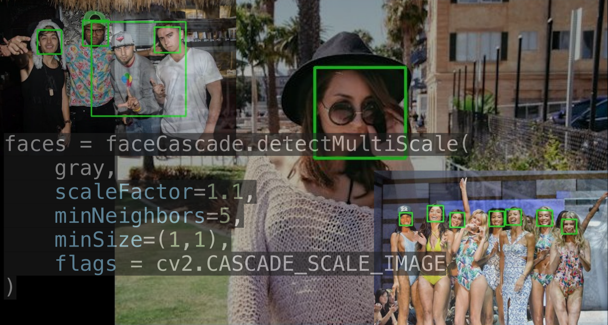 I’m writing this blog assuming that you have no prior knowledge of Machine Learning . Now, let’s talk about face detection. Face detection is finding one or many faces in a picture or a video. So, How do we find those faces? Well, we can use deep learning. Right? But actually the approach that everyone uses isn’t Deep Learning and it was developed in the early 2000s! Before deep learning was “a thing” to do everything :p, people used create algorithms with small neural networks, using machine learning and classifiers etc. and face detection was ongoing research at this time. In the year 2002, Paul Viola and Micheal Jones came up with a paper called ”Rapid Object Detection using a Boosted Cascade of Simple Features”. Here’s a link to the paper https://www.cs.cmu.edu/~efros/courses/LBMV07/Papers/viola-cvpr-01.pdf Here, I’ll attempt to explain their method in a simplified manner as to give you an insight to the concept of Haar cascades. Despite the fact that deep learning has taken over everything, this algorithm works absolutely fine till date! And if you have any kind of camera that does some sort of face detection, it’s probably using something very similar to this algorithm. 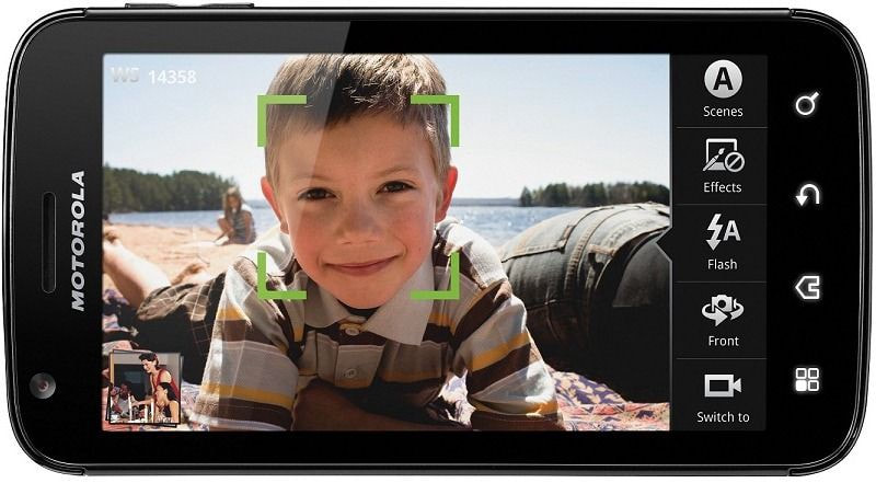 So what does this algorithm do? There are a few problems with face detection.
There’s a trade-off between accuracy and speed, false positives and false negatives and other constraints which makes it difficult to find faces quickly. Some other problems include the age, ethnicity, accessories such as if a person is wearing glasses etc. Viola-Jones came up with a classifier that uses very simple features that is one bit of an image, subtracted from another bit of an image. Unlike Deep learning which takes edges and other features and combines them together into objects, in a hierarchy and maybe it finds faces, what the Viola-Jones method does is it makes very quick decisions about what it is to be a face. \o_o/ For e.g. if you look at your own gray scale image, your eyes are arguably slightly darker than your forehead in terms of shadows and the pupils being darker. 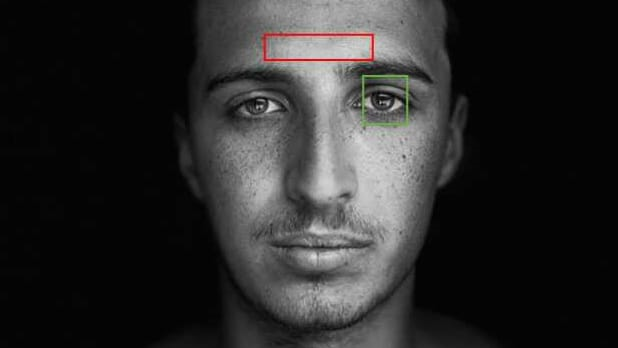 Hence the value of the image in the red rectangle subtracted from the value of the image in the green rectangle will produce a new different matrix. On its own this classification is very weak as it would also detect any other part of the image or in an different image where a certain section of the image is lighter than some other section. But if we could produce a lot of these all at once and make a decision that way. They proposed these simple rectangle features that subtracts one part of an image from another part. One of such features is a two rectangle feature. 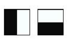 Voila-Jones algorithm is a machine learning approach. Since there can be many, say 500 faces in an image so we put in some features calculated from the image and we use machine learning to classify bits of the image or the whole image. Their contribution was a very quick way to calculate this features and use them to make a face classification. 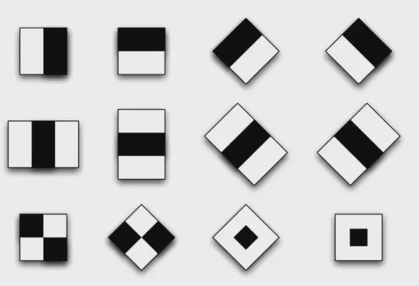 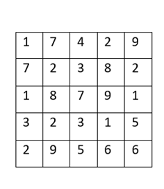 Their algorithm has a training process that selects certain features out of the many that makes sense in a particular section of the image i.e. to select the features that are useful. For e.g. a feature would be relevant over the eyes only and not anywhere else. Another problem is, on an image calculating large groups of pixels and summing them up is quite a slow process. So they came up with an idea called an integral image which makes this way faster. Suppose the given matrix is an image. (This is a very small image o_0,) Weight matrixSuppose we want to use the two-rectangle feature we previously discussed about : 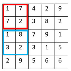 Suppose we want to use the two-rectangle feature we previously discussed about : Subtracting the blue block from the red block. That would be very simple: (Sum of the pixels in the red box) — (Sum of the pixels in the blue box) = (7+7+1+2) — (8+3+1+2) But, if you are doing this on a large section of an image and thousands of time this won’t work. Viola-Jones came up with Integral image where we pre-compute some of the arithmetic, store it in an intermediate form and then we can perform the rectangle feature function on it. 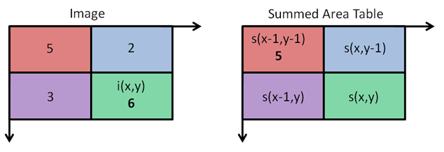 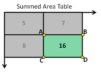 So we do one pass over the image, and every new pixel is the sum of all the pixels above and to the left and including it. Example of summed area table : For our image matrix 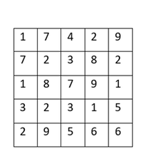 Integral Image would be 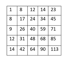 for eg: 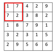 Sum of these 4 pixels 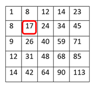 I’ll suggest you to do it for yourself , to understand it better. You’ll notice that in our sample image the sum of all the pixels is 113. 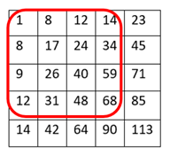 For e.g. the sum of the 4x4 block is 68 .So if we want to find the value of this region here 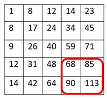 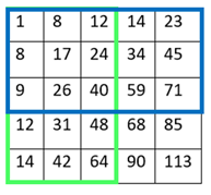 We would need to subtract the green box and the blue box.  And add this bit, since it was subtracted twice.therefore, it would be 113–64–71+40 = 18 6+6+1+5 =18Since it’d be doing huge amount of calculations at once, the integral image is calculated once and then used as a base to do really quick adding and subtracting of regions. How does this turn into a working face detector? lets image we are detecting a face. In this particular algorithm we are looking at 24x24 pixel regions, but they can be scaled up or down a little bit. The algorithm calculates all 180,000 possible combinations of 2,3,4 rectangle features for that 24x24 pixel and work out which ones for the given data set (of faces and not faces), best separates the positives from the negatives. 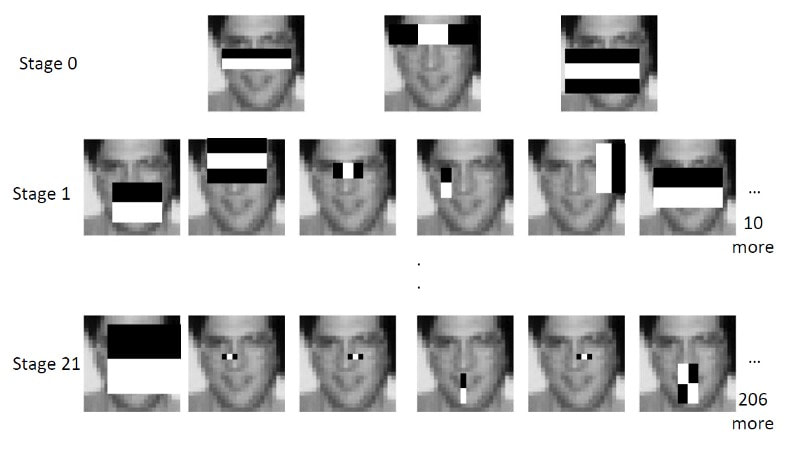 For e.g. In the image above, If all the features at stage 0 seem plausible, we let it through. If it fails to qualify in any of the three features in stage 0 we fail that region of the image. If stage 0 passes, we let it through the next stage. Which means the regions that passed the 0th stage, could be a face (but are definitely not NOT A FACE). Then all the regions that pass the 0th stage go through the stage 1 set of features and all the regions that pass through stage 1 go to stage 2 and so on. This is called a “Degenerate decision Tree.” Every time we calculate one of these features it takes little bit of time. The quicker we can say “no definitely not a face “, the better. And the only time we need to look through all these features (or all of the good ones) when we think that there actually could be a face in that region. So we can say less general, and more specific features go forward right up to about the number where we find a fail. And if we make it all the way to the end and nothing fails, that’s a FACE! Face Recognition using pre-trained Haar cascade classifiers. Here is a git-hub link to for various pre-trained Haar cascade classifiers https://github.com/opencv/opencv/tree/master/data/haarcascades These cascades are basically .xml files consisting of a lot of feature sets, and these feature sets correspond to a very specific type of object. Here, I’ll show you how to use some of these cascades and later we would discuss on how to make your very own cascade. We will be using the haarcascade_frontalface.xml and haarcascade_eye.xml files. Download these two files in the same project you would be writing your code in. import numpy as np import cv2 #Loading the two cascade files face_cascade=cv2.CascadeClassifier('haarcascade_frontalface.xml') eye_cascade=cv2.CascadeClassifier('haarcascade_eye.xml') cap =cv2.VideoCapture(0) while 1: ret, img = cap.read() gray=cv2.cvtColor(img,cv2.COLOR_BGR2GRAY) faces=face_cascade.detectMultiScale(gray, 1.3, 5) for (x,y,w,h) in faces: cv2.rectangle(img,(x,y),(x+w,y+h),(255,0,0),2) roi_gray = gray[y:y+h, x:x+w] roi_color = img[y:y+h, x:x+w] eyes = eye_cascade.detectMultiScale(roi_gray) for (ex,ey,ew,eh) in eyes: cv2.rectangle(roi_color,(ex,ey),(ex+ew,ey+eh),(0,255,0),2) cv2.imshow('img',img) k = cv2.waitKey(30) & 0xff if k == 27: break cap.release() cv2.destroyAllWindows() I’ll link a YouTube tutorial for the same. https://www.youtube.com/watch?v=88HdqNDQsEk Creating Your own custom Haar Cascade classifier A detailed step by step discussion on creating a Haar cascade has been discussed in this paper from University of Auckland (Link below), I do recommend you to try this approach on your own. https://www.cs.auckland.ac.nz/~m.rezaei/Tutorials/Creating_a_Cascade_of_Haar-Like_Classifiers_Step_by_Step.pdf I will also link a YouTube tutorial which uses Linux and AWS for training at a very low cost. https://www.youtube.com/watch?v=jG3bu0tjFbk But here, we will be discussing the more simple ,GUI approach for training which requires less time comparatively too. An Iranian developer named Amin Ahmadi has built this GUI (link) http://amin-ahmadi.com/cascade-trainer-gui/ That you’d be required to download. Now we need data sets for training there are many sources to find data sets, or you call simply download from google images. for face detection we will be using ck data set http://www.consortium.ri.cmu.edu/ckagree/  you need to form two folders n for negatives and p for positives. The p folder should contain all positives, in this case our positives will be faces. 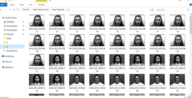 and the n folder should be negatives, in this case images with strictly no faces 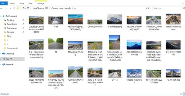 Once the data sets have been created you need to mention the path location of the data sets  Make sure that the data sets are named n and p. On the common tab, we can change the number of stages. With more number of stages, the time for training also increases but the model becomes more accurate too, in this case to train about 150 images 15 stages will be fine.  Keep the rest of the parameters at default.
On the cascade tab, you can change the width and the height, which is set at 24 (default). If you are using the ck data set, the images are bigger in size so we will set both sample width and sample height to 32. Keeping all the rest of the parameter at default, you can start the training process. Once the training is completed, you’ll see a classifier folder generated in your directory, which will contain a cascade.xml file. You can now import that file in your program and test your classifier. I strongly recommend you to try to create you own custom classifiers and test it. Also do visit the links and the tutorials for better understanding.
0 Comments
The AICVS club hosted a competition based on Deep learning and computer vision on the Kaggle interface on 6th October, 2019. The participants were supposed to submit their entries from 00.00 a.m. to 11.59 p.m., after solving the dataset remotely on their laptops. The dataset provided was--"MNIST dataset for handwritten numbers ", a well-known, accessible dataset.
This competition was mainly meant for students with a certain level of understanding of Deep learning and Computer Vision. However, students of all years were strongly encouraged to participate in the contest, regardless of their proficiency in the subject. To facilitate the same, the participants were sent video links, educating them about visualization of the concept, implementation and neural networks. This ensured that they were well-equipped to start working on the dataset smoothly. The participants were allowed to use any approach to solve the dataset, whichsoever they found convenient. To elaborate about the dataset, the MNIST dataset for handwritten numbers is a dataset containing tens of thousands of small square 28×28 pixel grayscale images of handwritten single digits between 0 and 9 . The task for the contestants was to train the network to classify a given image of a handwritten number into one of the 10 classes representing integer values from 0 to 9,inclusively. MNIST ("Modified National Institute of Standards and Technology") is the de facto “Hello World” dataset of computer vision. Since its release in 1999, this classic dataset of handwritten images has served as the basis for benchmarking classification algorithms. As new machine learning techniques emerge, MNIST remains a reliable resource for researchers and learners alike. The participants were supposed to submit their classification along with a copy of their Jupyter notebook to curb plagiarism. Although many people registered for the competition and attempted to solve the dataset, some of them could not submit the output file. However, this was an incredible opportunity for learners to get their feet wet in Computer Vision and play around with various approaches to solve a single dataset. The winners of the competition-- 1st: Atmaja Jape | Score : 0.98906 2nd: Bhavana Mache | Score : 0.97640 3rd: Aathira Pillai | Score : 0.97146 The winners were calculated by Kaggle on the private (tested on 70% of the test dataset) and public (tested on 30%of the test dataset) leaderboards and was shared with the hosts. They would be awarded e-certificates. The competition saw the maximum participation from the CS and IT branches. The content of the competition was highly rated and the students found it exciting and innovative. We received feedback saying that the contest was held in a proper manner and the club members assisted every participant having queries promptly. Although some students faced issues in the submission of the problem and the Kaggle Notebook crashed many times due to ram. We have surely taken a note on this and we will make sure that we take steps to manage this issue. Kaggle is a great place to learn and to participate in data science challenges. It has helped students learn a lot of new things. The 'learning by implementing' way is a fun way to learn and was greatly appreciated by the participants. The competition gave an insight to various parts of deep learning. It was like a hands-on demo where participants could actually visualize data and find appropriate solutions. All the participants are looking forward to another such innovative competition. We received a 100 percent response for students interested in participating in another AICVS Competition and we will host that really soon. Till then keep learning and keep practicing! Written by Shreya Abhyankar and Shreya Pawaskar. |
